Save Time in Excel with Autofill
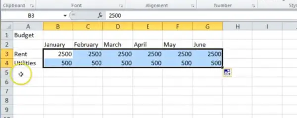
Autofill is one of our favourite Excel tools for saving time. In this two-minute video, Nicky explains how you can use Autofill when creating a small budget spreadsheet from scratch so you hardly have to type a thing!
Public Course Dates for Google Sheets Now Live

We have had lots of requests for Google Sheets, as many organisations (particularly charities and public sector) have made the switch to GSuite from Office 365.
How to Make Human Resources More Human

Tracey Waters is focused on improving employee experience at Sky UK. She has implemented two new practices: design thinking and agile methodology. The two processes compliment each other — design thinking is about problem finding, while agile is about problem solving.
In this full-length video from the 2019 Happy Workplaces Conference, Tracey explains how these two methodologies work together.
How to Extract First Names from Full Names in Excel Spreadsheets
If you are creating a Mail Merge using an Excel spreadsheet, this trick may help you. Often when downloading your data from your Client Relationship Management software or similar into a spreadsheet ready for a Mail Merge, you will find that both the first and last name are in the same column. In this blog, Henry explains how you can easily extract this information into two columns. Get in touch 020 7375 7300 Send us a message hello@happy.co.uk I seem to be sending a lot of merged emails lately and the source file for those emails generally contains the full name and the email, but not the first name. This is tricky as it is always nice to be able to say Hi Rosie, rather than just Hi or Hi Rosie Shepherd. And you can, because extracting the first name is fairly easy: Find the first space Step 1 is to find where the first space occurs, as this will normally be the end of the first name. Use the FIND function, which finds a character – or set of characters – in a cell, for this. This example finds the first space in A2: =FIND(“ “,A2) You can use the same technique for extracting first names from email, if the email format consists of firstname.surname@. In that case you search for the first full stop. Use the first space to find the first name You can then use the LEFT function, which takes the left most characters in a cell. Assuming here that the @FIND function has placed the position of the first space in C2. =LEFT(A2,C2-1) It is -1 because you don’t want to include the space itself. You can combine these two into one function like this: =LEFT(A2,FIND(“ “,A2)-1) What if some people have only entered a first name? If there is no space because they have only entered their first name, the above function will result in #VALUE! appearing. This can be fixed using the ISERROR function, which allows you to specify what happens if this function results in an error. We are assuming that the error results from there being only one word (the first name) in the name cell. So: This results in this function: =IF(ISERROR(FIND(” “,A2)),A2,LEFT(A2,FIND(” “,A2)-1)) If looking for a space in A2 results in an error, display A2. If there is a space, take all the characters up to the space. This function will work, as long as nobody has put Mr or Professor or similar in front of their name. And it also relies on the first name coming first, which isn’t true in all cultures.


