In his blog on Pivot Perfection, Darren showed us how to easily produce a series of Pivot Tables for each category we want to filter on. Slicers make it easy to have one Pivot Table that can switch between different categories.
Let’s start with the same data that Darren used:
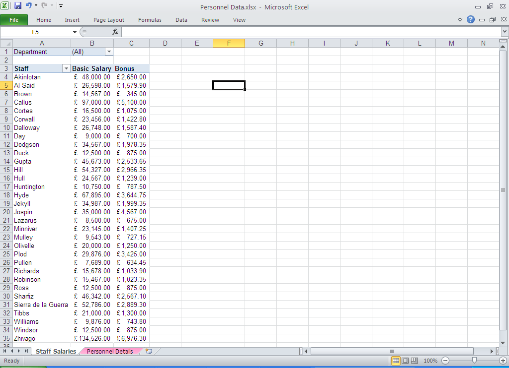
Example data
The next step is to add a Slicer:
1. Go to the Options tab of the Pivot Table Tools on the ribbon
2. Click on Insert Slicer
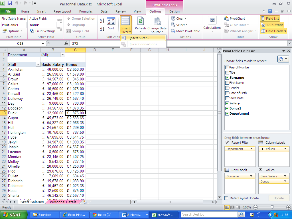
Insert Slicer option
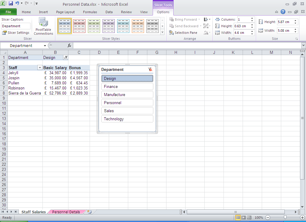
3.Choose the field you want to filter on, in this case Department
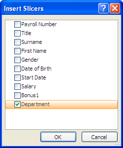
4. Click OK
5. A Slicer box will appear on your worksheet:
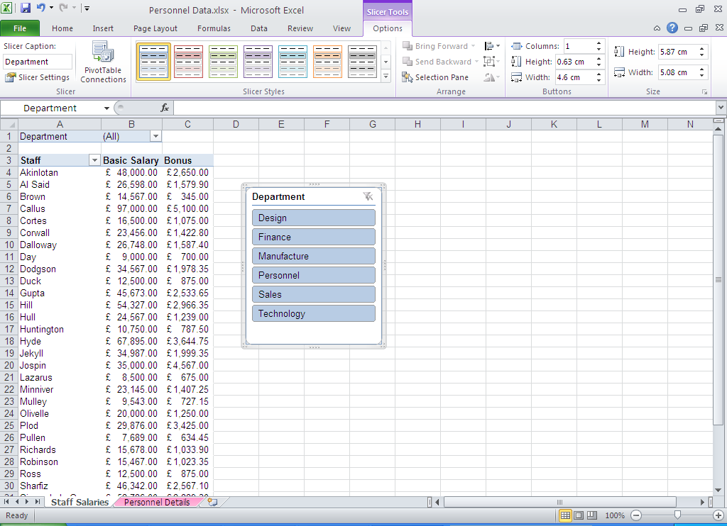
Example of a Slicer box
6. Click on the category you are interested in, for example, the Design department
7. The Pivot Table will update to show the values for that category:
8. To change to a different category, just click on the appropriate value in the slicer box
9. To select multiple values, do a normal click on the first value, then control-click on the other values:

Selecting multiple values
10. To clear the filter, click on the icon in the top-right corner of the Slicer box

Clearing your filter
11. You can move and re-size the Slicer box by clicking and dragging on the border of the box
Related Blogs
- How to Create a Pivot Table – If you’ve never used Pivot Tables before, start with this two-minute video.
- How to Group Dates Together in a Pivot Table – Learn how to group your data together by date in this short video.
- How to Use Pivot Tables in Excel to Create Sub-Reports – Another useful function of Pivot Tables that could save you time at work.